

On incentivizing anonymous participation

\cdot⋅
tl;dr; Blockchain activity is facilitated through independent actors participating in shared protocols. Incentivizing this participation is a critical design consideration, especially in permissionless, adversarial, and pseudonymous environments. We present a model and motivate the participation game in Section 1. In Section 2, we analyze this game’s symmetric, anonymous equilibria. We then apply this framework in two settings. Section 3 details prover markets, which aim to incentivize the generation of at least one proof. Section 4 turns to Proof-of-Work protocols, which aim to incentivize at least 50% participation (motivated by the goal of avoiding a 51% attack). In both cases, we derive the optimal incentive structure for the protocol to minimize its cost. We conclude in Section 5 by discussing how the model can be extended and other blockchain-specific techniques used for bootstrapping participation.
\cdot⋅
by maryam & mike – may 26, 2025.
\cdot⋅
Thanks to Akilesh, Noam, Matt, and Barnabé for review and discussion on this post!
Contents
(1). Motivation & Model
(1.1). Participation game model
(1.2). A trivial, non-anonymous solution
(1.3). A non-symmetric equilibrium
(2). Symmetric equilibrium of the lottery payment rule
(2.1). Considering large nn
(3). Prover market cost minimization
(3.1). Optimizing for at least one participant
(3.2). Asymptotics
(3.3). The 1 + \ln c1+lnc bound is tight
(4). A Proof-of-Work objective function
(4.1). Asymptotics
(5). Conclusion and future work
(5.1). Alternative cost functions
(5.2). Heterogeneous agents and information asymmetry
(5.3). Tokens, airdrops, and blockchain applications
1. Motivation & Model
Opening vignette – You are at your local sports bar and have a table to watch an NBA playoff game. You don’t want to watch alone, so you plan on letting the group chat know you are there. To make people more likely to come, you offer to buy the first round of wings, but you first need to decide how many to order. If you order too few, there is a chance no one shows up, thinking that someone else will go and there won’t be enough to go around. If you order too many, there won’t be room at the table if everyone comes. What is the optimal amount of wings to buy so that some, but not all, of your friends come?1
This story often comes up in blockchain protocol design. Protocols want to attract participation in some form and use incentives to elicit it:
- Proof-of-Work offers block rewards to incentivize miners to solve cryptographic puzzles.
- Proof-of-Stake offers consensus rewards for staking and voting correctly on blocks.
- Prover markets coordinate the production of computationally intensive ZK proofs.
Crucially, blockchains also want to allow permissionless participation. This makes the coordination problem much more difficult. This post presents a model for incentivizing participation and analyzes the symmetric equilibria of anonymous, common-value payment rules. In particular, we study the equilibrium where each player plays the mixed strategy of purchasing a lottery ticket with probability pp.
1.1. Participation game model
We model the participation game as follows:
- player – A player is a strategic agent who, based on the mechanism, can choose to purchase an entry ticket.
- participant – A participant is a player who purchases an entry ticket.
- protocol – The protocol is an agent with a cost function (or, equivalently, a positive valuation function) for inducing participation.
- payment rule – A function implemented by the protocol that maps the set of participants to their respective payments.
Let there be nn players in the participation game. Each faces the same entry fee, qq, making this a common-value auction. For simplicity, we use q=1q=1 for the remainder of this post. Each participant can deterministically decide to join or not; they can also choose to play a randomized strategy where they join with some probability pp. Before deciding whether to join, the participants observe a protocol-specified payment rule. The payment rule can depend on the realized set of participants and may be randomized. Each participant chooses an action to maximize their expected utility, meaning the expected payment they receive minus the entry fee (if they choose to participate).
The following two sections introduce the notions of anonymity and symmetry.
1.2. A trivial, non-anonymous solution
Suppose the protocol aims to attract at least one participant and assume players tie-break in favor of participation. A straightforward mechanism follows: “Choose a specific player, denoted WINNER, and tell them you will pay them $1 if they participate.” This trivial solution has many desirable properties:
- individual rationality for everyone (because each player can get utility zero by not participating), and
- satisfactory participation in equilibrium (
WINNERwill participate, and no one else will), and - payment minimization for the protocol (because $1 is the ticket fee, and thus the smallest possible cost for getting a participant).
If the protocol designer is OK with choosing a winner, then this solution is sufficient.2 Instead of stopping here, we focus on a set of solutions that are anonymous.
Definition (informal): An anonymous payment rule cannot depend on the identity of the player.
We formalize this property in Section 3.3, but hopefully, it should be intuitive. These payment rules must treat every player equally. The rules can depend on the players’ actions (e.g., by dividing the prize evenly among all participants that enter) and can be randomized (e.g., by giving the prize to a single participant randomly). However, the mechanism above relies on the player’s identity and is not anonymous.
1.3. A non-symmetric equilibrium
Separately, consider the following scenario: “A single player, denoted COMMITTER, makes a public commitment to purchasing a ticket and becoming a participant.” Depending on the payment rule, this commitment may disincentivize other players from participating. For example, suppose the payment rule evenly divides a prize of $1 between all participants. In that case, a second player considering joining is guaranteed negative utility because they pay $1 and earn $1/2. This leads to no one else joining the protocol and COMMITTER earning the full prize. This equilibrium is payment minimizing for the protocol but requires participants to pick COMMITTER, pushing the coordination complexity to the players. We use this example as motivation to restrict our attention to symmetric equilibria.
Definition: In a symmetric equlibirium each player use the same strategy.
This strategy can be deterministic (e.g., always buy a ticket and participate) or mixed (e.g., buy a ticket with probability pp). Since these deterministic strategies can be thought of as p=0p=0 or p=1p=1 respectively, any symmetric equilibrium is fully specified by a single value p\in[0,1]p∈[0,1]. In such an equilibrium, the number of participants is drawn from \text{Binomial}(n,p)Binomial(n,p), where nn is the number of players.
2. Symmetric equilibrium of the lottery payment rule
With our attention restricted to symmetric equilibria, there are only three outcomes for the players’ strategies:
- no one joins (p=0p=0),
- everyone joins (p=1p=1),
- everyone joins with probability p\in (0,1)p∈(0,1).
Depending on the payment rule, any of these outcomes is possible. This section studies the lottery payment rule.
Definition: A lottery payment rule pays a single player a prize of magnitude xx by uniformly randomly selecting a winner from the set of participants.
The lottery payment rule is anonymous and induces a symmetric equilibrium pp depending on the size of xx. The protocol sets the value of xx, the players decide whether or not to join, and the prize is given in full to one of the participants. If x<1x<1, we are in case (1); no one will join because the prize is less than the entry fee. If x\geq nx≥n, then we are in case (2); everyone will participate because they are guaranteed (in expectation) to be paid more than their entry fee. For other values of xx, the number of participants will be a random variable drawn from \text{Binomial}(n,p)Binomial(n,p) with p\in (0,1)p∈(0,1). The protocol can shift the mean, npnp, by tweaking xx.
We can characterize the symmetric equilibrium under case (3) above, where each player mixes their strategy and joins with probability pp. (There are many approaches to it; we show the explicit one here using differentiation; see Aside #1 for an alternative.) We consider player ii‘s decision by fixing the other players’ strategies at pp. ii chooses its joining probability p'p′ to maximize its expected utility,
In other words, player ii receives a payment of xx if she joins and wins the lottery among participants. In particular, since each of the other n-1n−1 players joins independently with probability pp, the number of participants beside ii is drawn from \text{Binomial}(n-1,p)Binomial(n−1,p). ii's utility from joining is that payout minus the ticket price. ii's utility from joining with probability p'p′ is her utility from joining times p'p′, since ii gets 0 utility from not joining.
For the symmetric strategy pp to be an equilibrium, p'=pp′=p must maximize this expression among all p'\in[0,1]p′∈[0,1]. The first order condition is
Setting this to zero, we get an analytical solution for the relationship between xx and pp,
This tells us: “given a prize of size xx, what probability pp creates a symmetric equilibrium” or equivalently, “if the protocol designer desires the participant count to come from \text{Binomial}(n,p)Binomial(n,p), they set a prize of size xx.” The plot below shows the relationship between these variables for n=2n=2.
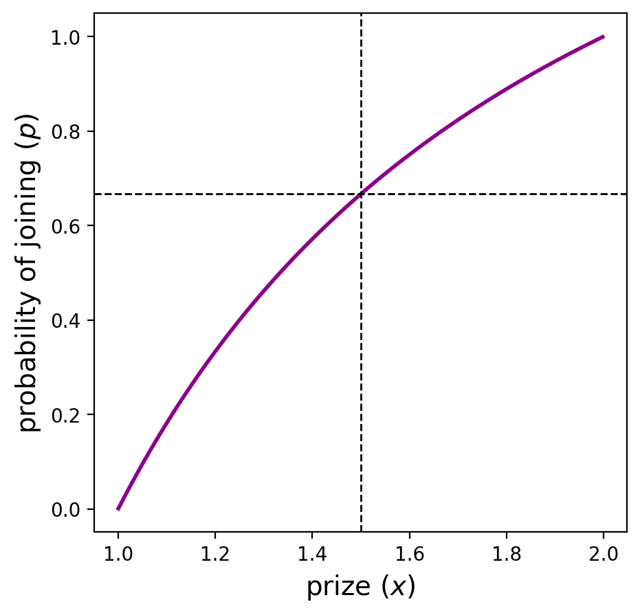
The dashed lines are interpreted as, “if the protocol sets the prize x=1.5x=1.5, then the strategy p=2/3p=2/3 is a symmetric equilibrium.” Also, notice that if the prize is <1<1 or >2>2, the players join with probability 0 or 1, respectively. These are the “no one joins” and “everyone joins” outcomes described at the beginning of this section. For the interior region, x \in (1,2)x∈(1,2), a unique pp is induced by each xx.
Aside #1 A different way of deriving the same equation is by considering the aggregate cash flow for the set of all players. For a given pp, the set of players pays npnp in expected entry fees. Thus, the protocol will need to pay npnp in expectation as reimbursement (because this is a competitive equilibrium, any excess value will be competed away). When the protocol chooses a prize xx, the set of players receives this prize as long as at least one player participates. This occurs with probability 1-(1-p)^n1−(1−p)n, meaning the set of players earn x \cdot (1-(1-p)^n)x⋅(1−(1−p)n) in rewards.
Aside #2: One interesting property of mixed-strategy equilibria is that the player is indifferent to either action (which is why they randomize their behavior in the first place). In the above example, if everyone else joins with probability pp, player ii receives zero utility from any action. You can see this by plugging in xx to her utility function,
\begin{align}U_i(p') &= \bigg[ x \cdot \frac{1-(1-p)^n}{np} -1\bigg] \cdot p' \\&= \bigg[\frac{np}{1-(1-p)^n}\cdot \frac{1-(1-p)^n}{np} -1\bigg] p' \\&= (1-1)p'\\&= 0.\end{align}[Math Processing Error]Another way of interpreting this is that the equilibrium is fully competitive. This induces the indifference between outcomes and the resulting mixed strategy.
2.1 Considering large nn
Recall the relationship
An interesting observation about this equation is that, for large nn, we can rewrite xx as a function of \mu=npμ=np (expected number of participants), using (1-x) \rightarrow e^{-x}(1−x)→e−x for small xx as
The protocol can target a desired mean participation count \muμ using this simple formula, without knowing nn. For example, if the protocol wants a single participant in expectation, it should set a prize of 1/(1-1/e)\approx 1.5821/(1−1/e)≈1.582. That is, the protocol pays a 58\%58% premium over the entry fee of 11 to attract one participant in expectation. This approximation improves as nn grows. The plot below shows the necessary protocol prize to attract one participant on average. It also shows the limit as n \to \inftyn→∞ approaches x(1)=1/(1-1/e)x(1)=1/(1−1/e).
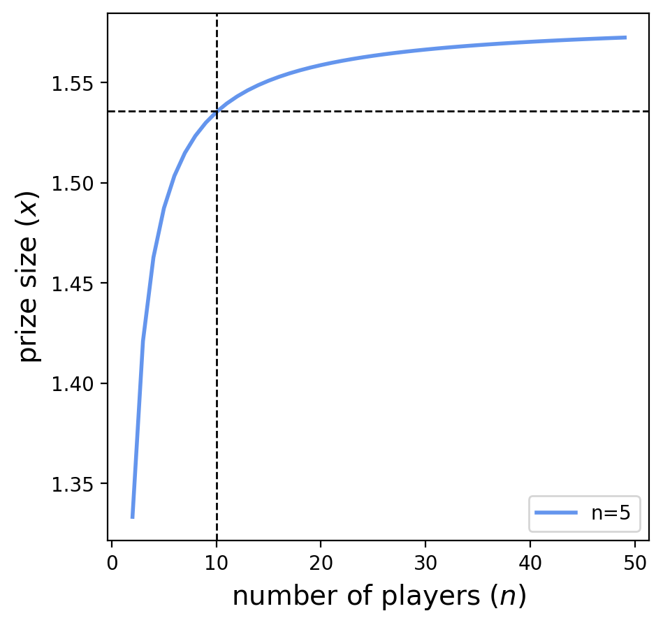
The dashed lines can be interpreted as: “if n=10n=10, then the protocol designer needs to set a prize of at least x=1.535x=1.535 to attract one participant in expectation.” Of course, the protocol designer may choose a higher prize to reduce the risk of no participants. The following section describes this tradeoff formally.
3. Prover market cost minimization
So far, we have shown how the protocol can target a specific expected participation count, \muμ, by varying xx. We now consider protocols that are particularly averse to low participation. We formalize this by introducing a “low-participation penalty.” In this section, we start by examining prover markets. In Section 4, we will look at a different low participation penalty motivated by Proof-of-Work consensus.
We consider a ZK rollup that wants to incentivize the costly production of proofs. The market designer may only care that at least 1 prover participates (and pays the entry fee, which is the cost of generating the proof).3 Further, say that if there is no participation at all, the protocol can generate the proof itself for a cost of cc (you can think of cc as the “outside option”). This allows us to write the low-participation penalty as a function of the number of participants, kk, as
Naturally, a protocol designer wants to choose the payment rule that minimizes its total cost (the prize size plus any penalty).
3.1. Optimizing for at least one participant
The analysis above allows the protocol designer to choose the magnitude of the prize to target a certain amount of participation under the symmetric equilibrium induced by the relationship between xx and pp. With the low-participation penalty, the protocol’s cost function, which we denote by C_pCp, is
This cost is what the protocol seeks to minimize, and the protocol faces a tradeoff when choosing xx when given cc. Too low of a value of xx results in the protocol incurring the penalty cc with high probability; higher values of xx are directly costly because the protocol has to pay a larger prize. Using the fact that in the symmetric equilibrium, each player participates with probability pp, we can write,
With x = \frac{np}{1-(1-p)^n}x=np1−(1−p)n (the relationship we derived above), this simplifies to
This is the protocol cost, which it seeks to minimize over p \in [0,1]p∈[0,1]. With the optimal probability p^*p∗, the protocol can directly calculate the prize size needed to induce the symmetric equilibrium at p^*p∗. We minimize the protocol’s cost using the first-order condition,
The second derivative is always negative over p \in [0,1]p∈[0,1], so p^*p∗ is indeed a unique local minimizer of the protocol cost. The following plot shows the protocol cost as a function of xx (which has a bijection with p\in(0,1)p∈(0,1)) for n=2n=2 and c=1.5,2,2.5c=1.5,2,2.5, respectively.
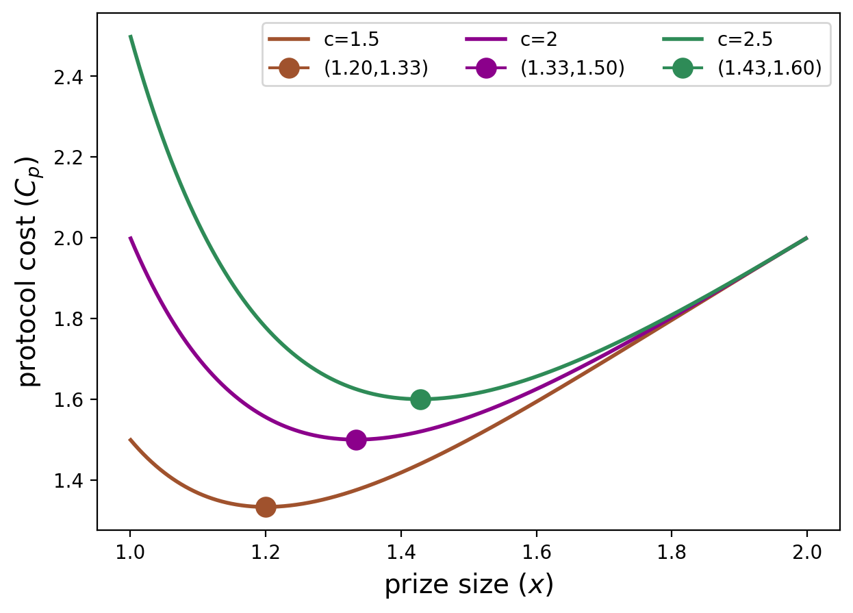
The x^*x∗ values (denoted as dots in the plot) are increasing in cc because as the protocol faces a higher penalty for no participation, it chooses higher x^*x∗ (which results in a higher p^*p∗) to be very confident that at least one player will participate. From p^*p∗, we calculate the optimal prize size in closed form as
We also calculate the optimal protocol cost of
The plot below helps visualize this cost as a function of n,cn,c.
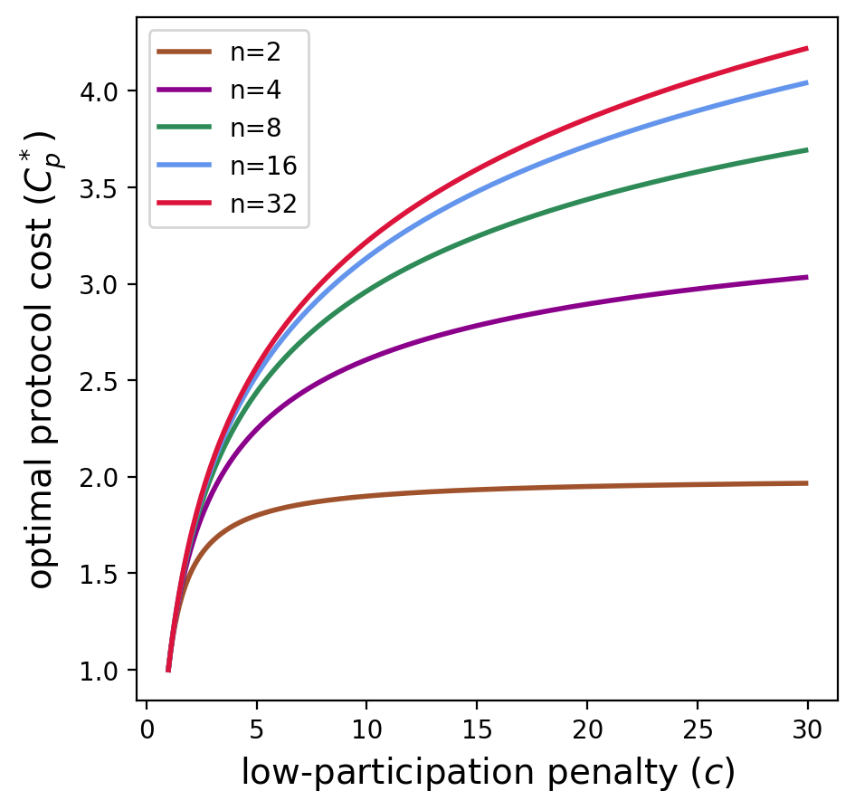
We see that as the low-participation penalty increases, the protocol cost seems to scale logarithmically. The next section formalizes this relationship by looking at the asymptotic behavior of the protocol cost.
3.2 Asymptotics
A natural question arises about how the values of p^*, x^*, C_p^*p∗,x∗,C∗p scale as a function of cc. In particular, a protocol designer may want to know how their utility scales as a function of cc assuming a large number of players in the game, nn. Expanding (see footnote4 for derivation), we get
Similarly, we can examine the asymptotic behavior of x^*x∗ (see footnote5 for derivation), which is the optimal prize for the cost-minimizing protocol:
Finally, we examine the asymptotic behavior of the optimal cost paid by the protocol, C_p^*C∗p (see footnote6 for derivation):
Critically, we see that as n\to\inftyn→∞, the total cost of the protocol scales as 1+ \ln c1+lnc. This is great for the protocol because it provides a logarithmic bound on the cost as a function of the outside option. Further, the optimal cost doesn’t depend on nn. This is nifty in a permissionless setting because the protocol can set an optimal prize just based on the quality of the outside option (i.e., the low-participation penalty) without knowing how many players there are! It also means the protocol can be sure their costs are bounded even if the number of players in the game is very large.7
The next section answers the question, “can we beat this logarithmic bound?” More formally, does an anonymous payment rule exist such that the resulting symmetric equilibrium has a protocol cost C_p < 1+\ln cCp<1+lnc? We show in the following section that the answer is no! The protocol cost is tightly bounded by 1+\ln c1+lnc.
3.3 The 1+\ln c1+lnc bound is tight
Note for the math/formalism-averse crowd: this section can be safely skipped!
We know that each player joins with probability pp in the symmetric equilibrium. We need to formalize the anonymity property we sketched in Section 1.2 to compare our mechanism with other anonymous payment rules. A payment rule \pi(S,r)π(S,r) takes as input the set S\subseteq [n]S⊆[n] of participants that joined and a random seed rr, and outputs a payment to each participant. The mechanism in the previous section pays a random participant the lottery prize xx with probability 1/|S|1/|S| if SS is non-empty and pays no one otherwise. We say a mechanism \pi(S,r)π(S,r) is (ex-post) anonymous if it’s pointwise symmetric with respect to the agent’s actions. Formally, \piπ is ex-post anonymous if for all rr and SS and all permutations \sigmaσ, \pi(S,r)=\pi(\sigma(S),r)π(S,r)=π(σ(S),r). When a mechanism is anonymous, we can rewrite its payment rule as \pi(S,r)=\pi(k,r)π(S,r)=π(k,r) where k=|S|k=|S| and is drawn from \text{Binom}(n,p)Binom(n,p). We now only care about the number of participants rather than the specific set.
Let \pi(k,r)π(k,r) be an anonymous mechanism with a symmetric equilibrium pp. Then, the expected cost to the auctioneer is
This expectation is taken over the randomness realization, rr, and each possible number of participants, kk. In expectation, we know that each of the kk participants must be individually rational to join the lottery. In aggregate, any protocol must pay at least each participant’s entry fee in expectation. Formally, \mathbb{E}_{k,r}[\pi(k,r)] \geq np.Ek,r[π(k,r)]≥np. Plugging this in, we again arrive at the form
At equality, this is exactly the protocol cost for the lottery mechanism. So it has the same optimal protocol cost of C_p^* = n-(n-1) c^{-1/(n-1)}C∗p=n−(n−1)c−1/(n−1) and asymptotic behavior of 1+\ln c1+lnc as n \to \inftyn→∞ apply. The lottery mechanism is optimal among anonymous and individually rational mechanisms in minimizing the “at least one player” objective!
4. A Proof-of-Work objective function
In the previous section, the protocol incurred the cost cc only if there was no participation, corresponding to the following step function in the number of participants, kk,
This cost function makes sense for the prover market example, where a single participant is necessary because only a single proof will suffice to satisfy the protocol. In other blockchain contexts, different low-participation penalties (or general participation valuation functi


